Maintenance teams report MTTR, MTBF, and availability every month. The numbers go into dashboards, leadership reviews, and capital planning decks. But too often, these metrics are analyzed in isolation. A technician team celebrates a 15% reduction in MTTR, while reliability engineers notice MTBF has dropped 20% on the same asset class. Operations sees 98.5% availability and assumes everything is on track, while maintenance knows that number is being held up by expedited shipping costs and weekend overtime.
These three metrics are not independent. They are mathematically bound, and changes in one directly affect the others. Understanding that relationship—how a shift in repair time influences uptime, or how failure frequency impacts spare parts demand—is what separates reactive reporting from proactive maintenance planning.
This guide walks through how to calculate each metric correctly, how to interpret them together, and how to use that correlation to make better decisions about labor, inventory, preventive strategy, and capital replacement.
The Mathematical Link Between MTTR, MTBF, and Availability
MTTR (Mean Time To Repair) is the average time required to restore an asset to operational status after a failure. MTBF (Mean Time Between Failures) is the average operating time between functional failures. Availability is the proportion of time an asset is capable of performing its intended function.
The relationship is straightforward:
Availability = MTBF / (MTBF + MTTR)
This formula is useful because it forces a practical question: if availability is below target, is the constraint failure frequency or repair duration? The answer determines where you invest. Reducing MTTR requires better diagnostics, parts staging, or technician training. Extending MTBF requires improved preventive maintenance, condition monitoring, or component upgrades. Trying to improve both without understanding which is the limiting factor wastes budget and effort.
One nuance: this formula assumes a single asset in a series configuration with no redundancy. In parallel systems or facilities with backup equipment, operational availability will be higher than the calculated inherent availability. That’s not an error—it’s a reminder that context matters. Always clarify which type of availability you’re measuring before drawing conclusions.
Why Isolated Metric Tracking Leads to Misaligned Decisions
Tracking MTTR, MTBF, and availability separately creates blind spots. Here are common patterns we see in the field:
- MTTR improves, MTBF declines: Repairs are faster, but failures are more frequent. This often means technicians are applying temporary fixes instead of addressing root causes. The metric looks good short-term; reliability degrades long-term.
- MTBF improves, MTTR increases: Assets fail less often, but when they do, repairs take longer. This can signal increased system complexity, aging components requiring specialized skills, or spare parts that are harder to source.
- High availability with high cost: Uptime targets are met, but only through expedited shipping, contractor overtime, or redundant equipment. The metric is achieved, but the total cost of ownership is unsustainable.
- Fleet-wide averages masking local issues: A 95% availability target across 50 locations might hide three sites running at 80% while the rest compensate. Without segmentation, poor performers never get the attention they need.
How to Calculate MTTR, MTBF, and Availability Accurately for Maintenance Decisions
Accurate calculation of MTTR, MTBF, and availability starts with clean data and consistent definitions. Small errors—like using calendar hours instead of runtime, or excluding parts lead time from repair duration—can distort trends and lead to misaligned maintenance strategies. This section breaks down the correct formulas, common pitfalls, and practical adjustments to ensure your metrics reflect operational reality, not just spreadsheet math.
Mean Time To Repair (MTTR)
Formula: Total downtime hours ÷ Number of repairs
MTTR should include the full restoration timeline: fault detection, diagnosis, parts procurement, repair execution, testing, and return to service. Excluding administrative delays or parts lead time creates an artificially low MTTR that doesn’t reflect operational reality.
Example: A pump fails at 8 AM. Diagnosis takes 2 hours. The required seal is not in stock; procurement takes 18 hours. Repair and testing take 3 hours. Total downtime: 23 hours. MTTR for this event is 23 hours, not 5. If your system only logs “wrench time,” you’re missing the bottleneck.
Mean Time Between Failures (MTBF)
Formula: Total operational hours ÷ Number of failures
Use actual runtime hours, not calendar time. A conveyor running two shifts daily accumulates wear differently than one used intermittently. Also, MTBF assumes a constant failure rate, which applies best to the “useful life” phase of the bathtub curve. For assets in infant mortality or wear-out phases, consider Weibull analysis or trending failure intervals instead of a simple average.
Tip: Segment MTBF by failure mode. A compressor might have high MTBF for mechanical failures but low MTBF for control system issues. Aggregating them hides the real problem.
Availability
Formula: (MTBF ÷ (MTBF + MTTR)) × 100%
Distinguish between:
- Inherent availability: Based on design reliability and maintainability (excludes preventive maintenance and logistics)
- Achieved availability: Includes preventive maintenance downtime
- Operational availability: Includes all delays—logistics, admin, external constraints
For maintenance planning, operational availability is most useful. It reflects what the business actually experiences. If operational availability is consistently lower than inherent availability, the gap points to supply chain, staffing, or workflow issues—not asset design.
How Correlating MTTR, MTBF, and Availability Reveals Hidden Maintenance Insights
Correlating MTTR, MTBF, and availability transforms raw maintenance data into actionable reliability intelligence. When these metrics are analyzed together, patterns emerge that isolated tracking cannot reveal—pointing directly to root causes, resource gaps, or strategy misalignments. Below are four real-world scenarios that demonstrate how metric correlation guides smarter maintenance decisions, from preventive optimization to capital planning.
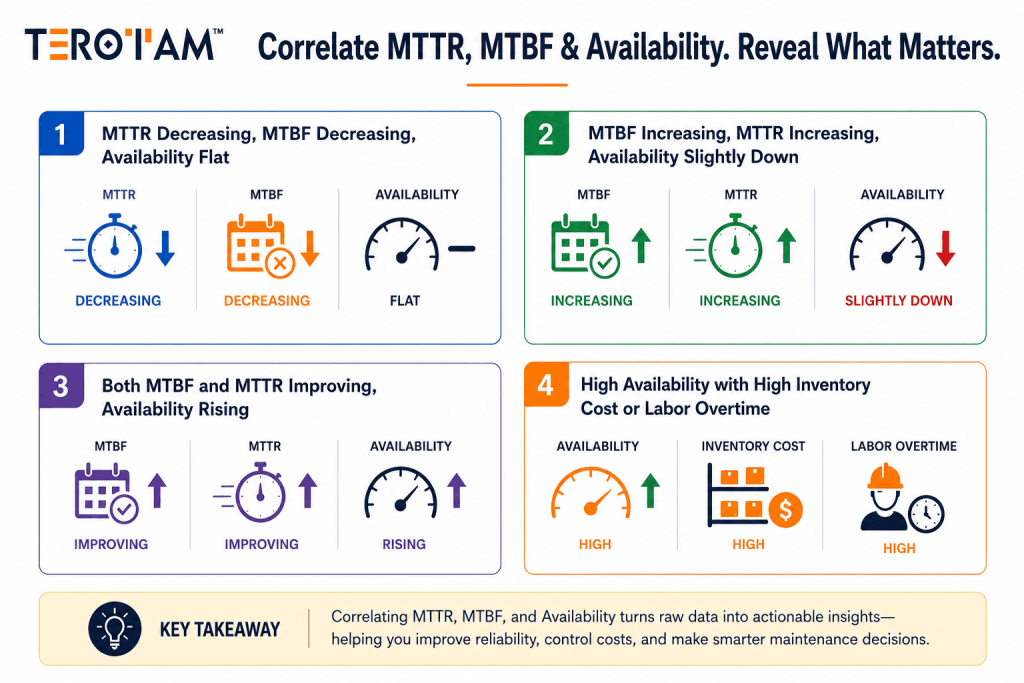
Scenario 1: MTTR Decreasing, MTBF Decreasing, Availability Flat
What the correlation signals: Repairs are getting faster, but equipment is failing more often. This pattern typically indicates a reactive maintenance culture where quick fixes replace root cause resolution, or preventive tasks are being deferred to meet short-term production targets.
Maintenance KPI correlation insight: A declining MTBF alongside improving MTTR suggests that failure frequency is the real constraint—not repair speed. The flat availability number masks underlying reliability decay.
Actionable next steps for reliability metrics:
- Audit recent work orders for repeat failure codes on the same asset or component
- Review PM compliance rates and adjust intervals based on actual runtime, not calendar dates
- Implement structured root cause analysis for failures that recur within 90 days
- Consider condition monitoring (vibration, temperature, oil analysis) to catch degradation before functional failure
Scenario 2: MTBF Increasing, MTTR Increasing, Availability Slightly Down
What the correlation signals: Assets are failing less frequently, but when they do fail, repairs take longer. This often points to increased system complexity, aging equipment requiring specialized skills, or spare parts that are no longer readily available.
MTTR vs MTBF analysis takeaway: The trade-off between fewer failures and longer repairs may still yield net operational benefit—but only if the extended downtime doesn’t impact production schedules or service commitments.
Actionable next steps for maintenance decision-making:
- Update spare parts strategy for critical, long-lead components; use usage data to optimize inventory turns
- Develop targeted technician training for complex repairs or newer equipment platforms
- Evaluate vendor service agreements for high-skill tasks that exceed in-house capability
- Model the cost impact: does reduced failure frequency offset the expense of longer downtime events?
Scenario 3: Both MTBF and MTTR Improving, Availability Rising
What the correlation signals: This is the ideal reliability trajectory. Preventive strategies are working, execution is consistent, and response times are optimized. The asset is both more reliable and more maintainable.
Reliability metrics for decision-making insight: When both leading indicators improve, availability gains are sustainable and cost-effective. This pattern validates current maintenance practices and supports strategic reinvestment.
Actionable next steps for asset availability optimization:
- Document the specific practices, intervals, or tools that drove improvement; standardize across similar assets
- Use the positive trend to justify extending replacement cycles or reallocating budget to other priority assets
- Share success metrics with leadership to secure support for predictive maintenance or reliability engineering initiatives
- Continue monitoring for diminishing returns—eventually, further MTBF gains may require capital investment, not just maintenance optimization
Scenario 4: High Availability with High Inventory Carrying Cost or Labor Overtime
What the correlation signals: Uptime targets are being met, but the cost structure is unsustainable. Availability is being “bought” through expedited shipping, contractor overtime, or redundant equipment—not earned through genuine reliability.
Maintenance performance analytics dashboard insight: High availability alone doesn’t indicate healthy maintenance. Pair availability data with total cost of ownership, inventory turns, and labor utilization to see the full picture.
Actionable next steps for predictive maintenance KPIs:
- Calculate total cost of ownership for critical assets, including expedited parts, overtime labor, and downtime impact
- Optimize spare parts inventory using historical usage data and failure mode analysis
- Shift budget toward predictive maintenance technologies (IoT sensors, oil analysis, thermal imaging) to reduce failure frequency rather than just speeding up repairs
- Reevaluate redundancy strategy: is backup equipment justified by criticality, or is it masking poor reliability on primary assets?
Using Correlation to Prioritize Maintenance Investments
When MTTR, MTBF, and availability are viewed together, maintenance leaders can move beyond reactive reporting to proactive resource allocation. The correlation highlights whether the budget should flow toward technician training, parts inventory, preventive optimization, or capital replacement. It also provides defensible data for leadership discussions—showing not just what happened, but why it happened and what to do next.
For teams using a CMMS, this analysis becomes scalable. Automated data capture, structured failure coding, and real-time dashboards make it possible to correlate metrics across dozens or hundreds of assets without manual spreadsheet work. The result is maintenance planning grounded in evidence, not intuition.
Common Calculation and Interpretation Errors
- Using calendar hours instead of runtime for MTBF: Skews results for intermittently used equipment. Always use meter readings or PLC data when available.
- Excluding diagnostic or logistics time from MTTR: Creates an unrealistic view of restoration capability. If parts lead time is consistently the longest portion of downtime, that’s a supply chain issue, not a technician performance issue.
- Averaging across dissimilar assets: Combining data from critical production equipment and auxiliary support systems masks localized reliability issues. Segment by asset tier, system, or criticality.
- Ignoring censoring in MTBF calculations: Assets that haven’t failed during the observation period still contribute operational time. Excluding them underestimates MTBF. Use proper reliability analysis methods when working with incomplete failure data.
- Treating metrics as static targets: MTBF and MTTR should inform continuous PM adjustment. If a component’s MTBF is trending down, the preventive interval may need adjustment. If MTTR is rising for a specific failure mode, the repair procedure may need revision.
How TeroTAM’s CMMS Supports Accurate Metric Tracking
Reliable correlation depends on consistent, accurate data captured at the source. TeroTAM’s CMMS is structured to reduce manual tracking errors and provide clear visibility into how MTTR, MTBF, and availability interact.
- Automated runtime and downtime logging: Operational hours and repair durations are captured directly from work order execution, reducing calculation drift from manual entry.
- Structured failure coding: Standardized failure modes link repairs to root causes, enabling MTBF analysis by component, system, or asset tier.
- Mobile execution with timestamp verification: Technicians record accurate start/stop times, parts used, and task completion status in the field, ensuring MTTR reflects actual restoration timelines.
- Asset hierarchy and criticality segmentation: Metrics are filtered by location, system, and criticality level, preventing misleading fleet-wide averages.
- Configurable reliability dashboards: MTTR, MTBF, and availability are displayed with trend lines, threshold alerts, and comparative views across sites or shifts.
- Predictive alerting: When MTBF trends downward or MTTR exceeds baseline for a critical asset, the system flags the shift for maintenance review before availability degrades.
- Export-ready reporting: One-click reports provide leadership, compliance, and finance teams with verified reliability data to support budget approvals, capital requests, or vendor evaluations.
A Practical Framework for Using Correlation in Maintenance Planning
- Establish baselines by asset tier: Calculate current MTTR, MTBF, and availability for critical equipment using 6–12 months of historical data. Segment by location, system, or criticality as needed.
- Identify the primary constraint: Determine which metric is furthest from target and whether the gap is driven by failure frequency, repair duration, or external factors like parts availability.
- Map interventions to the constraint:
- MTTR gap: Focus on diagnostics training, parts staging, or repair procedure standardization
- MTBF gap: Optimize PM intervals, implement condition monitoring, or address component quality
- Availability gap: Evaluate redundancy, logistics, or scheduling adjustments
- Model the impact: Use the availability formula to project outcomes. If MTTR drops by 20%, what does availability become? If MTBF improves by 15%, how does spare parts demand change?
- Prioritize by criticality and ROI: Focus resources on Tier 1 assets where metric improvements directly impact production, safety, or customer experience.
- Review and adjust: Track metric shifts monthly, refine PM intervals quarterly, and recalibrate targets annually based on actual performance data.
Conclusion
MTTR, MTBF, and availability are interconnected indicators, not independent scores. Reading them together reveals whether maintenance efforts are preventing failures, resolving them efficiently, or simply managing symptoms with overtime and expedited parts. Correlation turns maintenance data into a practical tool for budget allocation, capital justification, and continuous improvement.
When teams stop chasing isolated KPI targets and start analyzing how these metrics influence each other, downtime becomes predictable, costs stabilize, and asset performance aligns with operational goals.
To learn how TeroTAM’s CMMS suite can support accurate, correlated reliability tracking across your asset portfolio, contact us at contact@terotam.com.